I’m a bit of a geek when it comes to Excel/Google Sheets. Don’t get me wrong, there are many formulas that make my eyes cross. Excel, yes, math…not so much. But Excel does math for me so I don’t have to be good at math. Thank you Excel! When I come up with something I feel is useful for librarians, I try and share it with other librarians. I can’t tell you how many times I’ve heard back something along the lines of, “Thank you, I’ve just never felt comfortable with Excel, but this is going to be so useful!” So today I’m covering one of my favorite tools, Excel. And why it’s actually really useful for librarians!
Tracking sheets. These are so useful once I have them set up, because I can keep an eye on my numbers, see comparisons, and when my director needs numbers as the fiscal year draws to a close, I don’t have to think about it or agonize for hours. My two most commonly used is one for tracking my collection development budget, and my program attendance. For reference, here’s my current Program Attendance Tracking Sheet that everyone at my library uses for all age groups. This is a little different then the one I’ve sent out on ARSL before, primarily because I’ve added in Community since my new library likes to track numbers for community events even if we can’t use them in our program numbers. Anyways, I’m not here to talk about that, but if you want to ask me any questions about it, get the original Excel version without Community events, or just make a copy of the google sheet and save it for yourself, feel free!
In the meantime, I’m going to use something simpler for my example, a book budget tracking sheet. Here’s some example data, very plain. I always add in a Notes section because sometimes I can’t remember what something was for, but that’s personal preference.
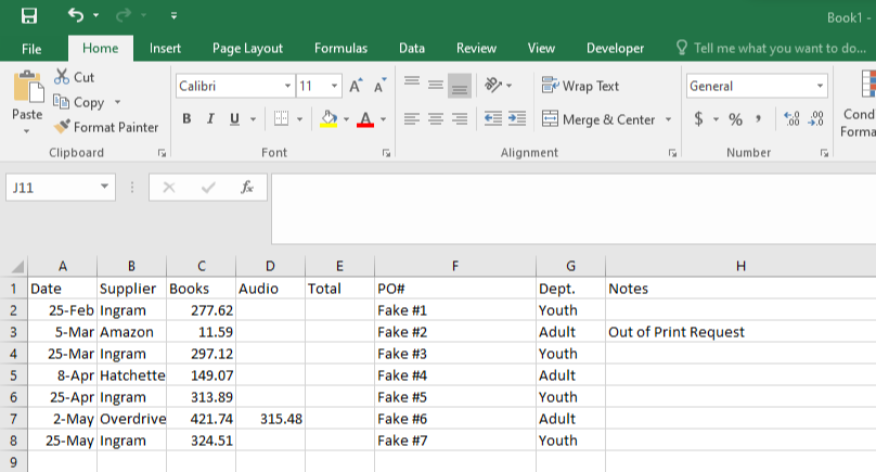
I’m going to assume you have some Excel basics under your belt, like how to refer to a particular cell (for example, E2 reference the cell that is on the E column on row 2), that you can type in =5+5 and Excel will tell you the answer’s 10, and that you can select cells and hit AutoSum to see what they all add up to. Today, my focus is on the formulas I use most heavily in my Excel projects: COUNTIF and SUMIF. COUNTIF counts how many time there is an occurrence of something. For instance, if I wanted to count how many times there was an order placed in the Youth department, it would be easy enough to count in a sheet with not much data—4 times in this sheet. But that number won’t automatically update as you add more. And when you have a multitude of lines, counting get really obnoxious. The point of Excel is to let it do the heavy lifting, after all.
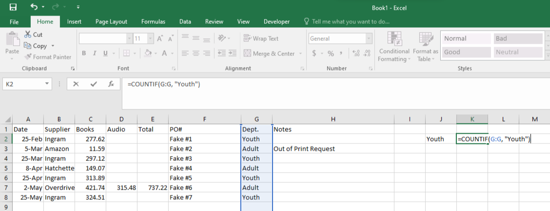
So I put in the equal, COUNTIF, an open parenthesis, then the range. For the purposes of this worksheet, I wanted all of column G, because that is where the data I’m wanting counted is located. You can either hit the G at the top of the screen, or type G:G. If you wanted a specific data range, that could be G2:G25, for example. Then the comma and your criteria, in this instance “Youth”. It’s searching text, so you need the apostrophes around it. And don’t forget a closing parenthesis so Excel knows you’re done! When I press enter, it told me 4. When I put in a new line, it automatically added it in like so:

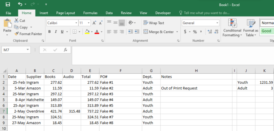
I went ahead and added in an adult column for sake of being a completionist. Now, maybe you don’t care about the exact number of orders the Youth Dept. makes versus Adult, but what if you wanted to count how many Ingram orders were made? Or in a programs tracking sheet, how many programs were inperson versus virtual? Or, just the other day, I downloaded my list of books I was considering buying from Ingram and added in a column so I could put in which specific age range each was in, so I knew how many I had in the cart for each age group. Counting would have been obnoxious, but after a couple minutes I had how many Board/Picture/Easy Reader/Chapter/Kids/YA books I had in the order and as I trimmed down by deleting particular line, those formulas automatically updated. Presto, I didn’t overbuy/underbuy for a particular section!
In summary, think of COUNTIF as Excel counting how many times something is happening IF a particular criteria is met. I love love love COUNTIF, especially because I hate counting. For a more detailed explanation, go to this link. Microsoft Office has really upped their game when it explaining things. If you want to learn something about anything in Microsoft Office, get the name (hovering over the button if needed) and search it on Microsoft’s support site. They have listings for practically everything.
Onwards to SUMIF! So, if COUNTIF counts occurrences, it follows that SUMIF does the same thing but with sums, right? Pretty much, but you’re adding another column in. Say instead of wanting to know how many purchases each department has made so far, you instead want to know how much each has spent.

Breaking this formula down, you’re still wanting data from column G (is this line earmarked as Youth?), but instead you’re telling Excel, “Does column G have Youth in it? If so, add the number from E into the total!” That’s why it’s =SUMIF(G:G, “Youth”, E:E). This gives you how much money the Youth dept. has spent on collection development so far:
Now that you’ve done that, you want it Adult’s totals too, right? Here’s a trick. Instead of typing it all again, click into the cell with the formula you want to copy.

See that green square? When you hover over that, a + sign will appear. When you drag it down, it copies that formula down into the next cell. Of course, it’s still adding up the Youth purchases, so you just go into the formula bar above, change “Youth” to “Adult”, and you’re good to go! Here’s the link to the SUMIF article on Microsoft’s support website.
You won’t believe how much weight the COUNTIF and SUMIF formulas can carry. If I’m making a tracking sheet, I’m using at least one of those formulas, probably both, and many times over. Now, warning. If a formula is looking for a particular line of text, whatever’s in quotation marks, you can’t make spelling mistakes or use alternative words. Case won’t matter, but if you’re in a hurry and type in yuth it’s not getting added in. Make sure you type things in correctly, OR add in Data Validation. Go to the Data Tab and find Data Validation. Highlight the column that you’re worried about then hit Data Validation.

As you can see, I’ve hit the dropdown menu under Allow, and have List highlighted. An option to type in a list of text will come up under Source, and you can type the options into that box. In this, that would be Youth, Adult. Just the words you want and a comma between each item. This will add a dropdown menu in each cell, but more importantly, if the wrong thing is typed:

A small addition, but useful for those of us who make mistakes in a hurry.
Ok, take a break. Play around with Excel, or go do something completely frivolous! The rest of this is extra/building off of everything else.
Extras:
Don’t do your work twice! Once you’re happy with your sheet, save one copy as the master, and your year’s working copy as something else, such as FY 2022 Book Budget.
You can format an area as a table so that you get alternating colors on rows, which I always like visually. It also adds in some sorting options, like if you forgot to type something in and your stuff isn’t order by date anymore. Your date column in a table will have the option to sort alphabetically or reverse it, and presto, order has been restored! Or you want to look at a specific age group-sort by that column and everything will be clumped together.
Besides your main table, you could list your yearly budget for each department and add in formulas to track your spending and how much money is left. You could add in a section to track your spending by month, or track how much you’re spending on different materials.
You could start adding in multiple criteria with the plurals of COUNTIF and SUMIF, COUNTIFS and SUMIFS. On this sheet, for instance, you could see how many times the Youth Department ordered from Ingram, which would be: =COUNTIFS(G:G, “Youth”, B:B, “Ingram”)
Or how much was specifically spent in May with SUMIFS, which would look like:
=SUMIFS(E:E, A:A, “>=05/01/2022″, A:A,”<=05/31/2022”)
And if you wanted to see how much just the Youth department spent in May, like this:
=SUMIFS(E:E, A:A, “>=05/01/2022″, A:A,”<=05/31/2022”, G:G, “Youth”)
The breakdown on those formulas are the E:E is where you’re getting the total you’re adding up from, then the range for one criteria, the criteria, the range for the next criteria, and that criteria, etc. >= is greater than or equal to, <= is less than or equal to.
Formula not copying over properly? Excel assumes that a formula is using a relative reference-if the first row has =B4-B2, the next row will have C4-C2. If you need a cell reference not to change, add in dollar signs! If you put in $B$2 into a formula, that formula will also use whatever’s in B2! Learn more here.
Does your cell have a red triangle? Hover over it for Excel or Google Sheets to tell you what’s wrong with your formula. Sometimes, though, it’s because it just doesn’t have data yet. Excel knows you can’t divide by 0, for instance, so it will put an alert into the cell, but as you add data in later the red triangle will go away!
Adding in charts is actually pretty easy. Select the data you want to make a chart of, including the text that describes each section, and under the Insert tab select what kind of chart you want!
Make a tracking sheet for the year by making each sheet in the bottom a different month! Once you’re happy with what one month looks like, you can copy your sheet as many times as you want and just rename the sheets to the month in question. If you really want to get fancy, you can even add a yearly totals sheet at the end, and get numbers from other sheets by putting the sheet name followed by an ! then the cell name. Example, =October!B3 would bring the data from the October sheet into a cell on your new sheet.
Get a quick analysis of a weeding report or an overview of your collection with color coding! Download your report, open it in Excel, and click Conditional Formatting on the Home Tab on your selected column. From there, go to Highlight Cells Rules, and then you’ll have multiple options as to how to do a quick color code of your cells. You could highlight old Copyright Dates, how long ago something was added to the system, and/or how long ago something was checked out. I like using the three stoplight colors-green means it’s good, orange/yellow means it’s in the danger zone, and red is obviously bad. If you use that system on all three columns, you can quickly see where your problem books are.
Honestly, the best way to get a hang of it is to start simple and practice. Once you’re comfortable with one element, adding another element doesn’t feel as intimidating. COUNTIF and SUMIF are the same in Excel as Google Sheets. Google Sheets is useful for being free, and for allowing multiple people to access, though Excel has a few more bells and whistles. Sometimes uploading an Excel sheet to Google can mess with things a bit, though, so I suggest building your sheet in whichever one you intend to use. Here’s my example of our Budget sheet. It’s done in Google sheets because I work at a small library, and it’s just me and the Adult Services Librarian. There wasn’t much point in making two separate sheets, so this sheet was built around both our library’s needs. If you want to play around with any of my sheets, by the way, feel free to make a copy for yourself!
Excel and/or Google Sheets can be extremely useful for librarians. Once you have tracking sheets set up, all you have to do is add new entries as necessary, and otherwise forget it! It’s so much easier to give the needed numbers to our bosses when we can just open a sheet, or share the sheet with them directly. I’ve even used Google Sheets for programming before, a budgeting RP game I called Budget Busters. That’s an extreme example, but a class on Microsoft Office, especially Excel, can also be really useful for teens. Or just how to make their own budgets! It’s not a tool for every situation…but when you need it, what a difference it makes!